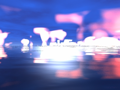
Lightflow C API sample ocean
- Lightflow
- by yuichirou yokomakura
- 2018.10.22 Monday 21:19
main6.cpp
#includeの両側に半角スペースが入っています。
$ /usr/local/gcc-2.95/bin/g++ -I ./include -lLightflow main6.cpp -o simplescene6
$ ./simplescene6
$ convert ocean.tga ocean.jpg
$ eog ocean.jpg
#includeの両側に半角スペースが入っています。
#include < Lightflow/LfLocalSceneProxy.h >
int main()
{
LfLocalSceneProxy* s = new LfLocalSceneProxy();
LfArgList list;
LfTransform trs;
// Specify some rendering settings. These values are used by
// all the built-in types, so they are grouped under a unique
// interface, named "default".
list.Reset();
list << "trace-depth" << LfInt( 5 );
list << "lighting-depth" << LfInt( 3 );
s->NewInterface( "default", list );
// Make a bright, bright light to model the sun.
list.Reset();
list << "position" << LfPoint( 0, 900, 100 );
list << "color" << LfColor( 60000.0, 60000.0, 60000.0 );
s->LightOn( s->NewLight( "point", list ) );
// Model the water waves with a fractal pattern.
s->TransformBegin( trs.Scaling( LfVector3( 10, 5, 5 ) ) );
list.Reset();
list << "basis" << "sin";
list << "scale" << 2.0;
list << "depth" << 0.1;
list << "turbulence.distortion" << 1.0;
list << "turbulence.omega" << 0.1 << 0.3;
list << "turbulence.lambda" << 2.0;
list << "turbulence.octaves" << LfInt( 5 );
LfInt waterbumps = s->NewPattern( "multifractal", list );
// the "basis" value describes the fractal basis, that here is set to
// "sin", as waves have a sinusoidal origin.
// "scale" represents the width of the waves. This factor is then
// multiplied by the scaling transform we put before.
// "depth" represents the depth of the waves, when used to displace a
// surface.
// the "turbulence." keywords are turbulence parameters, that are
// explained in the "multifractal" documentation.
s->TransformEnd();
// Model water with a material.
list.Reset();
list << "fresnel" << LfInt( 1 ) << LfFloat(0.3) << LfFloat(0.0);
list << "IOR" << 1.33;
list << "kr" << LfColor( 1, 1, 1 );
list << "kt" << LfColor( 1, 1, 1 );
list << "kd" << 0.0;
list << "km" << 0.03;
list << "shinyness" << 0.5;
list << "displacement" << waterbumps;
LfInt water = s->NewMaterial( "physical", list );
// the choosed type is "physical", because this provides physical
// parameters, very good to model liquids, glasses and metals.
// note the use of the waterbumps pattern as a displacement.
// Model the ocean fundals in a similar way.
list.Reset();
list << "basis" << "sin";
list << "scale" << 10.0;
list << "depth" << 0.5;
list << "turbulence.distortion" << 1.0;
list << "turbulence.omega" << 0.1 << 0.3;
list << "turbulence.lambda" << 2.0;
list << "turbulence.octaves" << LfInt( 5 );
LfInt earthbumps = s->NewPattern( "multifractal", list );
list.Reset();
list << "kr" << LfColor( 0.8, 0.75, 0.7 );
list << "displacement" << earthbumps;
LfInt earth = s->NewMaterial( "diffuse", list );
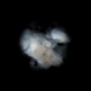
// Here starts the sky.
// It contains a lot of volumetric clouds, especially at the horizon,
// so it is a bit complex.
// Volumetric clouds are modeled with an interior and a pattern that modulates its density.
s->TransformBegin( trs.Scaling( LfVector3( 100, 100, 100 ) ) );
s->TransformBegin( trs.Translation( LfVector3( 0, 0, -0.5 ) ) );
list.Reset();
list << "value"
<< 0.0 << 1.0 << 1.0
<< 0.3 << 0.0 << 0.0;
list << "scale" << 1.0;
list << "turbulence.distortion" << 1.0;
list << "turbulence.omega" << 0.5 << 0.8;
list << "turbulence.lambda" << 2.0;
list << "turbulence.octaves" << LfInt( 3 );
LfInt cloudpattern = s->NewPattern( "multifractal", list );
// Make the output distribution go from 1 to 0.1 to model clouds.
s->TransformEnd();
s->TransformEnd();
list.Reset();
list << "kr" << LfColor( 2.0, 0.8, 0.4 );
list << "kaf" << LfColor( 0.6, 0.8, 0.4 ) * 0.035;
list << "density" << 1.0;
list << "density" << cloudpattern;
list << "sampling" << 0.07;
list << "shadow-caching" << LfPoint( -1000, -1000, -1 ) << LfPoint(1000, 1000, 100 );
list << "density-caching" << LfInt( 2048 ) << LfPoint( -1000, -1000, -1 ) << LfPoint( 1000, 1000, 100 );
list << "density-caching" << LfInt( 2048 ) << LfPoint( -1.2, -1.2, -1.2 ) << LfPoint( 1.2, 1.2, 1.2 );
LfInt cloudinterior = s->NewInterior( "cloud", list );
// Note that our scene will have a radius of 1000 unities, and our
// camera would be at its center, so with a sampling factor of 0.07 we
// allow 70 samples per ray: an enormous quantity! This will make our
// scene render slowly, but the caches will give a help. Obviously if
// you remove these volumetric clouds the rendering will be much faster.
// Here we don't care about speed however, since we want only to
// produce a single, astonishing image...
// Now model the fundal, a blue sky made of flat clouds that will be
// wrapped on a sphere.
list.Reset();
list << "color"
<< 0.2 << LfColor( 0.8, 0.9, 1.0 ) << LfColor( 0.8, 0.9, 1.0 )
<< 1.0 << LfColor( 0.2, 0.4, 0.9 ) << LfColor( 0.2, 0.4, 0.9 );
LfInt skypattern1 = s->NewPattern( "linear-v", list );
s->TransformBegin( trs.Scaling( LfVector3(80, 80, 10) ) );
list.Reset();
list << "color"
<< 0.2 << LfColor( 0.2, 0.4, 0.9 ) << LfColor( 0.2, 0.4, 0.9 )
<< 1.0 << LfColor( 0.2, 0.3, 0.7 ) << LfColor( 0.2, 0.3, 0.7 );
list << "scale" << 1.1;
list << "turbulence.distortion" << 1.0;
list << "turbulence.omega" << 0.5 << 0.8;
LfInt skypattern2 = s->NewPattern( "multifractal", list );
s->TransformEnd();
list.Reset();
list << "pattern" << skypattern1;
list << "gradient"
<< 0.3 << skypattern1 << skypattern1
<< 1.0 << skypattern2 << skypattern2;
LfInt skypattern = s->NewPattern( "blend", list );
// Note that we actually created two patterns, and we merged them
// together with a "blend".
// The first pattern is a linear gradient that will span the V
// direction of the parametric surface we will attach it to.
// In this case we will use it on a sphere, where the V direction is
// the one which connects the north and south poles (that is to say a
// line of constant U and varying V is a meridian).
// This gradient associates a color to each parallel of the sphere,
// going from bright blue near the horizon to dark blue near the
// azimuth.
// The second pattern is again a "multifractal", which we use to model
// very distant clouds. Note that we stretch it with a scaling, so that
// the clouds will look wide and thin.
// The "blend" pattern finally blends the two. It uses the pattern
// specified with "pattern" to mix more patterns. In particular it
// defines a pattern-gradient that smoothly interpolates between
// different patterns. In this case we use the linear pattern both to
// model the distribution of the gradient and to model the gradient
// itself.
// The numeric value of the linear pattern has not been specified
// (with a value-gradient), and so it goes from 0 to 1, as default.
// Thus the "blend" will make a transition that goes from a clear
// and bright sky near the horizon (at the V value of 0.3) to a cloudy
// sky near the azimuth (at the V value of 1.0).
// Create the sky material.
s->InteriorBegin( cloudinterior );
list.Reset();
list << "kc" << LfColor(1.0, 1.0, 1.0);
list << "kc" << skypattern;
list << "shadowing" << LfFloat(0.0);
LfInt sky = s->NewMaterial( "matte", list );
s->InteriorEnd();
// "matte" is a material made to create matte objects, that are not
// shaded by light, but that emit a uniform color. In this case this
// color is first set to white (1, 1, 1) and then scaled by the skypattern.
// The result will be the skypattern itself.
// Create a water disc.
s->MaterialBegin( water );
list.Reset();
list << "radius" << 1000.0;
s->AddObject( s->NewObject( "disc", list ));
s->MaterialEnd();
// Create an under-water disc made of earth.
s->TransformBegin( trs.Translation( LfVector3( 0, 0, -10 ) ) );
s->MaterialBegin( earth );
list.Reset();
list << "radius" << 1000.0;
s->AddObject( s->NewObject( "disc", list ));
s->MaterialEnd();
s->TransformEnd();
// Create the sky sphere.
s->TransformBegin( trs.Scaling( LfVector3( 1, 1, 0.1 ) ) );
s->MaterialBegin( sky );
list.Reset();
list << "radius" << 1000.0;
s->AddObject( s->NewObject( "sphere", list ));
s->MaterialEnd();
s->TransformEnd();
list.Reset();
list << "file" << "ocean.tga";
LfInt saver = s->NewImager( "tga-saver", list );
s->ImagerBegin( saver );
list.Reset();
list << "eye" << LfPoint( 0, -8, 4 );
list << "aim" << LfPoint( 0, 0, 4 );
list << "aa-samples" << LfInt( 2 ) << LfInt( 5 );
LfInt camera = s->NewCamera( "pinhole", list );
s->ImagerEnd();
s->Render( camera, 400, 300 );
delete s;
}
$ /usr/local/gcc-2.95/bin/g++ -I ./include -lLightflow main6.cpp -o simplescene6
$ ./simplescene6
$ convert ocean.tga ocean.jpg
$ eog ocean.jpg
- -
- -